Keywords: abundances, anomalous cosmic rays, Voyager, interstellar medium, heliosphere, solar wind termination shock.
A. C. Cummings and E. C. Stone
California Institute of Technology, Pasadena, CA 91125
We use energy spectra of anomalous cosmic rays (ACRs)
measured with the Cosmic Ray instrument
on the Voyager 1 and 2 spacecraft during
the period 1994/157-313 to
determine several parameters of interest to
heliospheric studies.
We estimate that the strength of
the solar wind termination shock is 2.42 (-0.08, +0.04).
We determine the composition of ACRs by
estimating their differential energy spectra at the shock
and find the following abundance ratios:
H/He = 5.6 (-0.5, +0.6),
C/He = 0.00048 ![]() 0.00011,
N/He = 0.011
0.00011,
N/He = 0.011 ![]() 0.001,
O/He = 0.075
0.001,
O/He = 0.075 ![]() 0.006,
and Ne/He = 0.0050
0.006,
and Ne/He = 0.0050 ![]() 0.0004.
We correlate our observations
with those of pickup ions to
deduce that the long-term ionization rate of neutral
nitrogen at 1 AU is
0.0004.
We correlate our observations
with those of pickup ions to
deduce that the long-term ionization rate of neutral
nitrogen at 1 AU is ![]() and that the charge-exchange cross section for neutral
N and solar wind protons is
and that the charge-exchange cross section for neutral
N and solar wind protons is ![]() at 1.1 keV.
We estimate that the neutral C/He ratio
in the outer heliosphere is
at 1.1 keV.
We estimate that the neutral C/He ratio
in the outer heliosphere is
![]() .
We also find that heavy ions
are preferentially injected
into the acceleration process at the termination shock.
.
We also find that heavy ions
are preferentially injected
into the acceleration process at the termination shock.
Keywords: abundances, anomalous cosmic rays,
Voyager, interstellar medium, heliosphere, solar wind termination shock.
Anomalous cosmic rays (ACRs) are energetic particles which are thought to be accelerated pickup ions. The main acceleration is thought to take place at the solar wind termination shock (Pesses et al., 1981). The source of the pickup ions that become ACRs is believed to be neutral gas from the interstellar medium (Fisk et al., 1974). The ACR component currently consists of seven elements: H, He, C, N, O, Ne, and Ar (Garcia-Munoz et al., 1973; McDonald et al., 1974; Hovestadt et al., 1973; Cummings and Stone, 1988, 1990; Christian et al., 1988, 1995; McDonald et al., 1995). Previous studies of their composition have led to estimates of the abundances of neutral gas in the interstellar medium (Cummings and Stone, 1987, 1990). However, those studies were made before the pickup ion observations became available and the fractionation in the acceleration and propagation processes could only be roughly estimated.
In this study we adopt a new approach that makes use of the pickup ion observations and the ACR observations to gain information on the injection of the pickup ions into the acceleration process at the termination shock. This approach has only become viable as solar modulation has lessened to such an extent that the observed ACR energy spectra are less modulated than at any time in the past. This decreased modulation results in ACR spectra which show signs of a power-law dependence at low energies, which makes possible estimates of the ACR spectra at the shock.
The ACR shock spectra are estimated for H, He, C,
N, O, and Ne.
Ar, which was included in previous studies, is
observable only at energies above the roll-off
energy of the shock spectrum.
Thus we can gain no information on the low-energy
power-law portion of the shock spectrum, which
is what is required for this study.
Estimates of the neutral densities of
H, He, N, O, and Ne in the outer
heliosphere (30 - 60 AU) are available
from pickup ion studies
(Geiss et al., 1994; Geiss and Witte, 1996).
We use a model of their ionization and
subsequent transport to estimate the fluxes of pickup
ions incident on the termination shock.
We use a theory of
particle acceleration at the termination shock to estimate
the resulting power-law differential energy spectra
for these elements.
These spectra can be compared with
our derived ACR shock spectra
to estimate the relative injection efficiencies of
pickup ion ![]() ,
,
![]() ,
,
![]() ,
and
,
and ![]() .
We do not have independent information on the charge-exchange cross
section of N, so in the case of N we can
estimate this quantity and the ionization rate of N at 1 AU
by using an estimate
of the injection efficiency of pickup ion
.
We do not have independent information on the charge-exchange cross
section of N, so in the case of N we can
estimate this quantity and the ionization rate of N at 1 AU
by using an estimate
of the injection efficiency of pickup ion ![]() based on that
of
based on that
of ![]() and
and ![]() .
Also, by using an estimate
of the injection efficiency
of
.
Also, by using an estimate
of the injection efficiency
of ![]() , we can estimate the neutral C abundance
in the outer heliosphere.
, we can estimate the neutral C abundance
in the outer heliosphere.
In order to estimate the ACR shock spectra,
we compare our observations made with the
Cosmic Ray instrument
(Stone et al., 1977) on
V1 and V2 during 1994/157-313
with a spherically-symmetric equilibrium model of the propagation
of ACRs, including diffusion, convection, and adiabatic deceleration
(Fisk, 1971).
This period consists of three 52-day periods which
were part of a recent study on the distance to the
termination shock (Stone et al., 1996).
The average latitudinal gradient for ACR He
with 10 - 22 MeV/nuc was ![]() 0.8%/deg
for the period considered in that study, 1993/52 - 1994/365.
This latitudinal gradient is small enough
that we feel justified in using a
spherically-symmetric model of
propagation to make a first order estimate
of the shock spectra, shock location, and other
parameters. We will later make
a correction to the estimated shock location by accounting
for the finite latitudinal gradient.
0.8%/deg
for the period considered in that study, 1993/52 - 1994/365.
This latitudinal gradient is small enough
that we feel justified in using a
spherically-symmetric model of
propagation to make a first order estimate
of the shock spectra, shock location, and other
parameters. We will later make
a correction to the estimated shock location by accounting
for the finite latitudinal gradient.
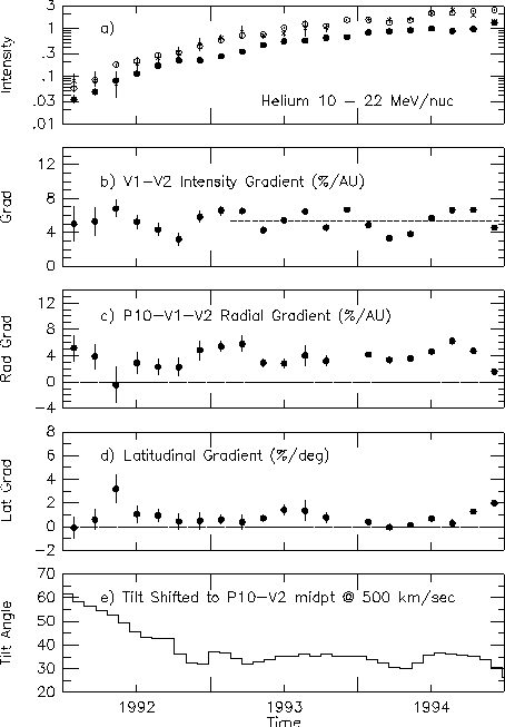
Figure 1:
Intensity of helium (52-day averages) measured
at P10 (crosses), V2 (solid circles), and V1 (open circles) versus time.
b) Intensity gradient between V1 and V2 for He
with 9.3 - 22.3 MeV/nuc. The dashed line is the
mean for the period indicated.
c) Radial gradient of ACR He with ![]() 10 - 22 MeV/nuc.
d) Latitudinal gradient of ACR He with
10 - 22 MeV/nuc.
d) Latitudinal gradient of ACR He with ![]() 10 - 22 MeV/nuc.
e) Estimated tilt of the neutral
current sheet shifted to the mid-point of V2 and P10.
Each tilt observation
(Hoeksema, private communication, 1995)
covers a single solar rotation or
10 - 22 MeV/nuc.
e) Estimated tilt of the neutral
current sheet shifted to the mid-point of V2 and P10.
Each tilt observation
(Hoeksema, private communication, 1995)
covers a single solar rotation or ![]() 26 days.
We have performed a 3-solar-rotation moving average on the
supplied tilt data set before plotting, in order to approximate the
average conditions between V2 and P10 which are
26 days.
We have performed a 3-solar-rotation moving average on the
supplied tilt data set before plotting, in order to approximate the
average conditions between V2 and P10 which are ![]() 17 AU apart.
17 AU apart.
Figure 1 is reproduced from Figure 2 of Stone et al. (1996) and displays the time history of He with 10 - 22 MeV/nuc, three gradients of these particles, and the tilt of the neutral current sheet. The time period we have chosen for this study, 1994/157-313, comprise the 4th through 6th 52-day periods of 1994 shown in panels a-d of Figure 1. In Figure 1b, intensity gradients between V1 and V2 are shown and it appears that the period 1994/157-313 chosen for this study has a larger than average gradient. The gradient for the period 1993/52 - 1994/365 is seen to wander about a mean value of 5.3%/AU showing no systematic increase or decrease. The non-statistical variations are caused by transient disturbances and ideally we would use a period that was unaffected by such disturbances, as was done in the Stone et al. (1996) study. However, in order to get good statistical precision for the heavier ACR species and to observe ACR H at both V1 and V2, it was necessary to use several of the most recent periods for the analysis.
By examining Figure 1a, we deduce that the transient disturbance during 1994/157-313 is affecting the V2 fluxes, making them lower than they would otherwise be. This atypical gradient can be accounted for in our model fits by moving the V2 spacecraft towards the Sun from its actual position and away from V1. Thus, the intensity we observe at V2 during this transient decrease is representative of the equilibrium intensity at a position some distance sunward of V2.
| Element | <T> |
|
|
|
| (MeV/nuc) | (%/AU) | (%/AU) | (AU) | |
| He | 20.1 | 4.49 | 5.32 | -2.41 |
| 26.0 | 2.69 | 3.37 | -3.26 | |
| 34.8 | 3.33 | 3.87 | -2.13 | |
| 43.9 | 2.07 | 2.40 | -2.12 | |
| O | 4.3 | 3.20 | 4.75 | -6.34 |
| 4.9 | 3.18 | 4.66 | -6.10 | |
| 6.2 | 3.25 | 3.91 | -2.64 | |
| 7.9 | 2.81 | 3.51 | -3.29 | |
| 10.5 | 2.91 | 3.52 | -2.71 |
In order to estimate the effective radial location
of V2, we examined the V1/V2 intensity gradients
in four He energy intervals and in five O energy
intervals for 11 52-day periods (1993/105 - 1994/313)
and for the period 1994/157-313.
We computed the distance, ![]() , to move V2 for each
energy interval from the equation:
, to move V2 for each
energy interval from the equation:
![]()
where ![]() is the average V1/V2 intensity gradient
for the 11 time periods,
is the average V1/V2 intensity gradient
for the 11 time periods, ![]() is the observed V1/V2
intensity gradient for the period 1994/157-313,
and
is the observed V1/V2
intensity gradient for the period 1994/157-313,
and ![]() and
and ![]() are the average
radial locations of the V1 and V2 spacecraft, respectively.
The average latitudes and radial locations of the
spacecraft
are 32.5
are the average
radial locations of the V1 and V2 spacecraft, respectively.
The average latitudes and radial locations of the
spacecraft
are 32.5 ![]() N and 56.8 AU for V1 and 12.3
N and 56.8 AU for V1 and 12.3 ![]() S and 43.7
AU for V2.
The gradients and radial shifts for V2 calculated
from Equation 1 are displayed in Table I.
We find that the average V2 correction
for the 9 observations is -3.4
S and 43.7
AU for V2.
The gradients and radial shifts for V2 calculated
from Equation 1 are displayed in Table I.
We find that the average V2 correction
for the 9 observations is -3.4 ![]() 0.5 AU.
Thus the effective radial location of V2 for the purposes
of the model fits is 40.3 AU.
0.5 AU.
Thus the effective radial location of V2 for the purposes
of the model fits is 40.3 AU.
In the model calculations
we fit the ACR H, He, C, N, O, and Ne spectra at V1 and V2.
These spectra are obtained by subtracting estimated
spectra of galactic cosmic rays from the observed spectra.
The estimated GCR spectra for each element were derived from the
observed C and O spectra at high energies.
For V1, a power-law fit, with the spectral index fixed at 1.0, was made
to three C intensity values with energies between 36 and 106 MeV/nuc.
Also in the fit was the highest energy O data point at 94 - 125 MeV/nuc,
scaled in intensity by the factor 1.095 to represent C.
The resulting V1 GCR C spectrum in units of
![]() was
was
![]() T,
where T is energy in MeV/nuc.
For V2, a similar fit was made, except a C data point
with energies 20 - 36 MeV/nuc was added to the fit.
The resulting V2 GCR C spectrum was
T,
where T is energy in MeV/nuc.
For V2, a similar fit was made, except a C data point
with energies 20 - 36 MeV/nuc was added to the fit.
The resulting V2 GCR C spectrum was
![]() T.
The assumed GCR abundances of the other species, relative to C,
are: 107, 35.6, 0.228, 0.913, and 0.132
for H, He, N, O, and Ne.
For N, O, and Ne, these ratios are from
Simpson (1983)
and represent observed GCR ratios at 70 - 280 MeV/nuc at 1 AU.
For He, we use the estimate from
Simpson (1983) at 600 - 1000
MeV/nuc.
For H, we estimate a ratio of GCR H/He = 3
from our observed V1 H and He energy spectra.
This ratio
is smaller than the value of 4.7
T.
The assumed GCR abundances of the other species, relative to C,
are: 107, 35.6, 0.228, 0.913, and 0.132
for H, He, N, O, and Ne.
For N, O, and Ne, these ratios are from
Simpson (1983)
and represent observed GCR ratios at 70 - 280 MeV/nuc at 1 AU.
For He, we use the estimate from
Simpson (1983) at 600 - 1000
MeV/nuc.
For H, we estimate a ratio of GCR H/He = 3
from our observed V1 H and He energy spectra.
This ratio
is smaller than the value of 4.7 ![]() 0.5 derived by
Simpson (1983).
0.5 derived by
Simpson (1983).
The ACR He
shock spectrum is assumed to be a power-law in energy per nucleon,
![]() .
The shock spectra of the other elements are assumed to
be a power-laws with the same index.
For O this is an adequate approximation for energies up to
.
The shock spectra of the other elements are assumed to
be a power-laws with the same index.
For O this is an adequate approximation for energies up to ![]() 10 MeV/nuc
and for ACR He this approximation is valid up
to
10 MeV/nuc
and for ACR He this approximation is valid up
to ![]() 60 MeV/nuc (see Stone et al. (1996) for
more discussion).
Above a total energy of
60 MeV/nuc (see Stone et al. (1996) for
more discussion).
Above a total energy of ![]() 150 - 240 MeV the energy spectra of these
elements exhibit
an approximately exponential roll-off
(Stone et al., 1996).
150 - 240 MeV the energy spectra of these
elements exhibit
an approximately exponential roll-off
(Stone et al., 1996).
We assume the diffusion coefficient,
![]() (in
(in ![]() ), is
given by
), is
given by
![]()
where ![]() and
and ![]() are scaling factors,
are scaling factors,
![]() is particle speed,
r is heliocentric radial distance in AU, and R is rigidity in GV.
This form was used by
Stone et al. (1996)
and can be derived from the quasilinear formulation of
Bieber et al. (1995).
There are ten free parameters in the model:
the shock location (
is particle speed,
r is heliocentric radial distance in AU, and R is rigidity in GV.
This form was used by
Stone et al. (1996)
and can be derived from the quasilinear formulation of
Bieber et al. (1995).
There are ten free parameters in the model:
the shock location ( ![]() ), the diffusion
coefficient scaling factor (
), the diffusion
coefficient scaling factor ( ![]() ),
the diffusion coefficient shape factor (
),
the diffusion coefficient shape factor ( ![]() ),
the power-law index (
),
the power-law index ( ![]() ) of the energy
spectrum at the shock, the intensity scaling factor (
) of the energy
spectrum at the shock, the intensity scaling factor ( ![]() )
of the
ACR He shock spectrum, and the ratios of the
intensity scaling factors of the other
elements to that of ACR He at the shock (H/He, C/He, N/He, O/He, and Ne/He).
We assume that the solar wind velocity, V, is 500
)
of the
ACR He shock spectrum, and the ratios of the
intensity scaling factors of the other
elements to that of ACR He at the shock (H/He, C/He, N/He, O/He, and Ne/He).
We assume that the solar wind velocity, V, is 500 ![]() ,
which is close to the average value at V2 of 490
,
which is close to the average value at V2 of 490 ![]() for 1993/1 - 1994/365 (Richardson, private communication, 1995).
The fits are not sensitive to
the actual value of V, but a different V would result
in a proportionally different
for 1993/1 - 1994/365 (Richardson, private communication, 1995).
The fits are not sensitive to
the actual value of V, but a different V would result
in a proportionally different ![]() .
.
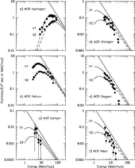
Figure 2:
ACR energy spectra at the positions of V1 and V2
spacecraft for the period 1994/157-313.
The curves represent the 10-parameter best-fit energy spectra at the
solar wind termination shock, V1, and V2, as described in the text.
a) ACR H,
b) ACR He,
c) ACR C,
d) ACR N,
e) ACR O, and
f) ACR Ne.
The data and best-fit model curves for the period
1994/157-313 are shown in Figures 2a-f.
The fits were made only in the energy regions shown
by the solid lines, below the exponential roll-off.
The ![]() of the ten-parameter best fit to
the 86 data points participating
in the fits in Figure 2 is 51.2.
Figure 3 shows the best-fit diffusion coefficient as
a function of rigidity.
of the ten-parameter best fit to
the 86 data points participating
in the fits in Figure 2 is 51.2.
Figure 3 shows the best-fit diffusion coefficient as
a function of rigidity.
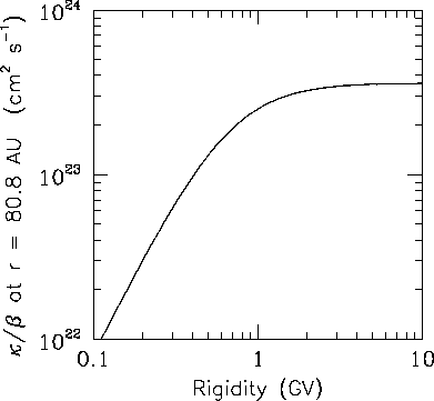
Figure 3:
Best-fit diffusion coefficient divided by particle velocity
versus rigidity at 80.8 AU. The form of the diffusion coefficient
is described in the text.
We investigated the confidence limits for each parameter in
two ways. We first estimated the 68% confidence limits
by iteratively changing and fixing the value of one parameter
and re-fitting until we found the parameter value where the ![]() had increased by 1 (see Press et al. (1992)).
We did this in turn for all ten parameters.
The best-fit parameter values and the
68% confidence limits are shown in
Table II for the period 1994/157-313.
had increased by 1 (see Press et al. (1992)).
We did this in turn for all ten parameters.
The best-fit parameter values and the
68% confidence limits are shown in
Table II for the period 1994/157-313.
|
Parameter | Fit | 68% | 68% | Model | Model |
| Value | Lower | Upper | Lower | Upper | |
| Limit | Limit | Limit | Limit | ||
| | -1.55 (-0.06, +0.03) | -1.62 | -1.53 | -1.56 | -1.55 |
|
| 80.8 (-3.0, +2.4) | 77.9 | 82.9 | 81.7 | 79.8 |
|
| 3.10 (-0.22, +0.17) | 2.92 | 3.22 | 3.23 | 2.98 |
|
| 1.51 (-0.09, +0.11) | 1.42 | 1.62 | 1.49 | 1.54 |
|
| 285 (-69, +81) | 217 | 366 | 288 | 279 |
| H/He | 5.6 (-0.5, +0.6) | 5.1 | 6.2 | 5.7 | 5.5 |
|
C/He ( | 4.8 ( | 3.7 | 6.0 | 4.8 | 4.9 |
|
N/He ( | 1.1 ( | 1.0 | 1.2 | 1.1 | 1.1 |
|
O/He ( | 7.5 ( | 7.0 | 8.1 | 7.5 | 7.7 |
|
Ne/He ( | 5.0 ( | 4.6 | 5.5 | 5.0 | 5.1 |
In the second method we account for modelling uncertainties by using the estimated uncertainty in the effective radial position of V2 (0.5 AU). We performed two additional fits, one using the upper limit for the effective radial location for V2 and another using the lower limit. The resulting parameters are shown as the model limits in Table II.
For the shock distance, we need to apply an additional correction to account for the small but finite latitudinal gradient. In the study by Stone et al. (1996), the authors took account of this effect by making a correction to the radial locations of V1 and V2 before using the spherically-symmetric model to fit the energy spectra. The correction they derived was
![]()
where
![]() is the effective location,
is the effective location, ![]() is the actual location,
is the actual location,
![]() is the average latitudinal gradient,
and
is the average latitudinal gradient,
and
![]() is the absolute value of the latitude of the spacecraft, and
where a model was used in which the radial gradient
in the intensity j is proportional
to 1/r, with
is the absolute value of the latitude of the spacecraft, and
where a model was used in which the radial gradient
in the intensity j is proportional
to 1/r, with
![]() .
In the current study, we make a correction to the radial
location of V2 to account for the transient intensity decrease
observed on V2.
The fits are then made with the actual V1 radial
location and the transient-decrease-corrected radial
location of V2.
Thus the resulting shock location,
.
In the current study, we make a correction to the radial
location of V2 to account for the transient intensity decrease
observed on V2.
The fits are then made with the actual V1 radial
location and the transient-decrease-corrected radial
location of V2.
Thus the resulting shock location, ![]() , is a first-order
estimate of the location if there were no latitudinal gradient.
To derive a correction factor to apply to
, is a first-order
estimate of the location if there were no latitudinal gradient.
To derive a correction factor to apply to ![]() ,
we assume that the ratio of intensities
at two locations can be described by
the following equation:
,
we assume that the ratio of intensities
at two locations can be described by
the following equation:
![]()
where ![]() is the intensity
at radial location
is the intensity
at radial location ![]() ,
C is the Compton-Getting factor,
V is the solar-wind speed, and
,
C is the Compton-Getting factor,
V is the solar-wind speed, and
![]() is the diffusion coefficient.
We assume that the diffusion coefficient
is proportional to radial distance,
is the diffusion coefficient.
We assume that the diffusion coefficient
is proportional to radial distance, ![]() ,
so that Equation 4 can be written
,
so that Equation 4 can be written
![]()
where ![]() and
and ![]() are the radial locations
where the intensities
are the radial locations
where the intensities ![]() and
and ![]() are measured, respectively.
Thus,
are measured, respectively.
Thus,
![]()
By applying Equation 6 for two cases: 1) ![]() and
and ![]() and 2)
and 2) ![]() and
and ![]() we find
we find
![]()
If we substitute the latitude-corrected spacecraft positions for the
actual positions, the best-fit shock position
should change such that the same shock flux ![]() and the fluxes
and the fluxes ![]() and
and ![]() are recovered.
Since
the right side of Equation 7
will remain unchanged, so must the left side.
That is,
are recovered.
Since
the right side of Equation 7
will remain unchanged, so must the left side.
That is,
![]()
and thus
![]()
From Equation 3,
![]()
and
![]()
By using these two equations in Equation 9, it can be shown that
![]()
where
![]()
Using Equations 10, 12, and 13, it can be shown that
![]()
where b = a - 1.
Using the values of ![]() %/deg,
and
%/deg,
and ![]() from
Stone et al. (1996),
and
from
Stone et al. (1996),
and ![]() AU from Table II, we find
AU from Table II, we find
![]() .
Applying this correction to the derived fit shock location
from Table II, we find
.
Applying this correction to the derived fit shock location
from Table II, we find
![]() AU.
We caution, however, that this estimate is based on Equation
5 which is only an approximation to the solution of the
full transport equation.
No systematic error to account for this source
of uncertainty has been added.
AU.
We caution, however, that this estimate is based on Equation
5 which is only an approximation to the solution of the
full transport equation.
No systematic error to account for this source
of uncertainty has been added.
The shock strength (see, e.g.,
Potgieter and Moraal (1988)),
s, is related to the spectral index by:
![]() .
From the values of
.
From the values of ![]() in Table II, the inferred strength
of the shock
is 2.42 (-0.08, +0.04).
The shock is not a strong shock (s = 4;
in Table II, the inferred strength
of the shock
is 2.42 (-0.08, +0.04).
The shock is not a strong shock (s = 4; ![]() = -1),
a finding in agreement with the results from the
study by
Stone et al. (1996).
= -1),
a finding in agreement with the results from the
study by
Stone et al. (1996).
To estimate the efficiency ![]() for the injection of pickup ion
species i into
the acceleration process, we follow the calculations of
Lee (1983) from which it can be shown
that the accelerated spectrum is given in units of
for the injection of pickup ion
species i into
the acceleration process, we follow the calculations of
Lee (1983) from which it can be shown
that the accelerated spectrum is given in units of
![]() by
by
![]()
where ![]() for a downstream/upstream density ratio of 2.42,
for a downstream/upstream density ratio of 2.42,
![]() is the pickup ion flux
at the shock, and
is the pickup ion flux
at the shock, and ![]() is the injection energy
corresponding to 2
is the injection energy
corresponding to 2 ![]() ,
taken here to be
,
taken here to be ![]() MeV/nuc.
The pickup ion fluxes at the shock can be estimated
from the observations of
Geiss et al. (1994), who inferred the densities
of neutral H, He, C, N, O, and Ne in
the outer heliosphere shown in Table III.
Using these values, the model of
Vasyliunas and Siscoe (1976)
for the distribution of these neutrals throughout the
heliosphere, and the long-term ionization rates at 1 AU
from
Rucinski et al. (1996)
(also shown in Table III),
we estimate the fluxes of
MeV/nuc.
The pickup ion fluxes at the shock can be estimated
from the observations of
Geiss et al. (1994), who inferred the densities
of neutral H, He, C, N, O, and Ne in
the outer heliosphere shown in Table III.
Using these values, the model of
Vasyliunas and Siscoe (1976)
for the distribution of these neutrals throughout the
heliosphere, and the long-term ionization rates at 1 AU
from
Rucinski et al. (1996)
(also shown in Table III),
we estimate the fluxes of ![]() ,
,
![]() ,
,
![]() , and
, and
![]() pickup ions at the nose
of the heliosphere shown in
Table III and displayed in Figure 4.
We do not include the pickup ion fluxes of
pickup ions at the nose
of the heliosphere shown in
Table III and displayed in Figure 4.
We do not include the pickup ion fluxes of ![]() in Table III because the
neutral density of C from the pickup ion studies
is only an upper limit.
The
in Table III because the
neutral density of C from the pickup ion studies
is only an upper limit.
The ![]() pickup ion flux is also missing from Table III because
we could not find the charge-exchange cross section for N
and hence we could not independently estimate the
long-term ionization rate of N at 1 AU.
Later, we will use our observations to make estimates of
these parameters for N and of the neutral C
density in the outer heliosphere.
pickup ion flux is also missing from Table III because
we could not find the charge-exchange cross section for N
and hence we could not independently estimate the
long-term ionization rate of N at 1 AU.
Later, we will use our observations to make estimates of
these parameters for N and of the neutral C
density in the outer heliosphere.
| Element | Neutral abund. | Total ioniz. | Pickup ion |
| in outer | rate at | flux at nose | |
| heliosphere | 1 AU | of heliosphere | |
| ( | ( | ||
| H | | | 10240 |
| He | 1.00 | | 228 |
| C | | | |
| N | 0.5 (-0.3, +0.5) | ||
| O | 3.5 (-1.4, +1.8) | | 5.3 |
| Ne | 0.7 (-0.5, +1.0) | | 0.53 |
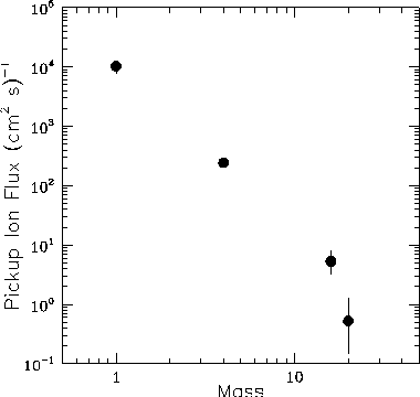
Figure 4:
Estimated fluxes of pickup
ions at the nose of the heliosphere at 100 AU,
the estimated location of the solar
wind termination shock.
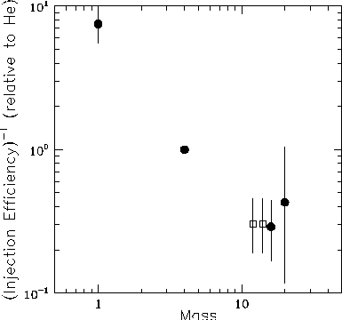
Figure 5:
Estimated injection efficiencies
of pickup
ions into the acceleration process
at the solar wind termination shock.
Equation 15 can be written:
![]()
where the coefficients ![]() are shown in Table IV.
These are the calculated ACR spectra
at the shock and they can be compared
with the derived ACR shock spectra from the model fits
(Figure 2) to derive the relative injection efficiencies
shown in Table IV.
The relative efficiencies are much more reliably
determined than the absolute efficiencies because
the uncertainty in the spectral index is removed when
the ratio is taken.
The estimated uncertainties in the relative injection
efficiencies include the uncertainties in the ACR
intensity scaling factors from Table II
and the uncertainties in the pickup ion fluxes,
which are assumed to be dominated by the uncertainties
in the neutral abundances from the pickup ion studies shown in
Table III.
It does not include any uncertainties associated with the
simplifications inherent in the acceleration model in Equation 15.
The relative injection efficiencies are shown as a function
of particle mass in Figure 5.
The observed preferential injection for the heavier
particles is qualitatively consistent with Monte Carlo
studies of shock acceleration by
Ellison et al. (1981)
but is in disagreement with the results of
Kucharek and Scholer
(1995).
are shown in Table IV.
These are the calculated ACR spectra
at the shock and they can be compared
with the derived ACR shock spectra from the model fits
(Figure 2) to derive the relative injection efficiencies
shown in Table IV.
The relative efficiencies are much more reliably
determined than the absolute efficiencies because
the uncertainty in the spectral index is removed when
the ratio is taken.
The estimated uncertainties in the relative injection
efficiencies include the uncertainties in the ACR
intensity scaling factors from Table II
and the uncertainties in the pickup ion fluxes,
which are assumed to be dominated by the uncertainties
in the neutral abundances from the pickup ion studies shown in
Table III.
It does not include any uncertainties associated with the
simplifications inherent in the acceleration model in Equation 15.
The relative injection efficiencies are shown as a function
of particle mass in Figure 5.
The observed preferential injection for the heavier
particles is qualitatively consistent with Monte Carlo
studies of shock acceleration by
Ellison et al. (1981)
but is in disagreement with the results of
Kucharek and Scholer
(1995).
| Element |
Coeff. |
| Inj. eff. | |
| from Eq. 16 | Table II | relative to He | ||
| H | | 1600 | | 7.5 (-2.5, +2.4) |
| He | | 285 | | 1.00 |
| O | | 21.4 | | 0.29 (-0.12, +0.15) |
| Ne | | 1.43 | | 0.43 (-0.31, +0.62) |
The open squares in Figure 5 represent weighted averages of
the inverse injection efficiencies for ![]() and
and ![]() .
They are plotted at mass mumbers 12 and 14
to represent the estimated injection
efficiencies of
.
They are plotted at mass mumbers 12 and 14
to represent the estimated injection
efficiencies of ![]() and
and ![]() .
For
.
For ![]() , the value plotted, 0.30 (-0.11, +0.15)
implies an absolute injection efficiency of 0.0174.
From Table II we estimate that the ACR N shock spectral intensity
coefficient is
, the value plotted, 0.30 (-0.11, +0.15)
implies an absolute injection efficiency of 0.0174.
From Table II we estimate that the ACR N shock spectral intensity
coefficient is ![]() which implies that
the coefficient
which implies that
the coefficient ![]() for N (
for N ( ![]() ) in Equation 16 is
3.1/0.0174 = 178.
) in Equation 16 is
3.1/0.0174 = 178.
![]() is proportional to the flux of pickup ions at
the shock.
By scaling from the flux of
is proportional to the flux of pickup ions at
the shock.
By scaling from the flux of ![]() pickup
ions at the shock from Table III, we find that the expected flux
of
pickup
ions at the shock from Table III, we find that the expected flux
of ![]() pickup
ions at the shock is 0.81
pickup
ions at the shock is 0.81 ![]() .
Using the model of
Vasyliunas and Siscoe (1976)
for the distribution of neutrals in the
heliosphere and the estimated neutral N density in
the outer heliosphere from Table III
(
.
Using the model of
Vasyliunas and Siscoe (1976)
for the distribution of neutrals in the
heliosphere and the estimated neutral N density in
the outer heliosphere from Table III
( ![]() ), we estimate
that the long-term ionization rate at 1 AU of neutral N
must be
), we estimate
that the long-term ionization rate at 1 AU of neutral N
must be ![]() .
This value is similar to that derived by
Rucinski et al. (1996)
for O
(
.
This value is similar to that derived by
Rucinski et al. (1996)
for O
( ![]() ).
).
For C, only an upper limit to the neutral abundance
in the outer heliosphere is available from the pickup ion observations.
We can supply an estimate of this abundance by using a
similar technique to that described above to deduce the ionization
rate of N at 1 AU, except that in this case we have the
long-term ionization rate of C from Table III
and the unknown is the neutral abundance of C in
the outer heliosphere.
If we assume the injection
efficiency for ![]() is as plotted in Figure 5,
it can be shown that the neutral C density
in the outer heliosphere must be
is as plotted in Figure 5,
it can be shown that the neutral C density
in the outer heliosphere must be
![]() ,
which implies the C/He ratio in the outer heliosphere
is
,
which implies the C/He ratio in the outer heliosphere
is ![]() .
The uncertainty is estimated from the uncertainty computed
for the injection efficiency for
.
The uncertainty is estimated from the uncertainty computed
for the injection efficiency for ![]() plotted in Figure 5
and the uncertainty in the neutral density of He in Table III.
The neutral abundances of all the elements are shown in Figure 6.
The abundances are plotted relative to He and for H, N, O, and Ne are
from the pickup ion observations
(Gloeckler, 1996; Geiss et al., 1994).
For C, we show two abundances which are in good agreement, one from this
study and one from
Cummings and Stone (1990) derived
from observations made during a solar minimum period in 1987.
plotted in Figure 5
and the uncertainty in the neutral density of He in Table III.
The neutral abundances of all the elements are shown in Figure 6.
The abundances are plotted relative to He and for H, N, O, and Ne are
from the pickup ion observations
(Gloeckler, 1996; Geiss et al., 1994).
For C, we show two abundances which are in good agreement, one from this
study and one from
Cummings and Stone (1990) derived
from observations made during a solar minimum period in 1987.
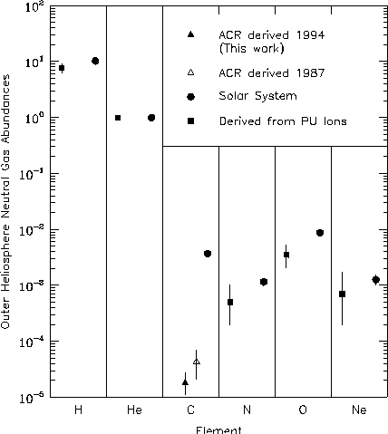
Figure 6:
Estimated abundances of neutral
gases in the outer heliosphere.
The solid squares are from pickup ion
studies (Geiss et al., 1996),
the solid circles
are solar system abundances (Grevesse and Anders, 1988),
and
the solid triangle is derived in
this study.
We consider the shock location derived from this study,
100 ![]() 6 AU, to be less accurate than the shock location
of 85
6 AU, to be less accurate than the shock location
of 85 ![]() 5 AU
derived for a slightly different period (1994/157-209) by
Stone et al. (1996).
The reason is that
the V1/V2 intensity gradients for the longer period considered
in this study are typically larger than the average.
Therefore, this period is likely affected by a transient or transients
that have decreased the intensity at V2.
While we have tried to take this into account by changing the
location of V2 for the fits, the previous study has an
advantage in that it used periods
when there were apparently no transients present.
We feel that the shock spectral
intensity ratios are relatively insensitive
to this effect and should be accurate.
As evidence of this we find that the O/He ratios derived
in the two studies are in good agreement.
We also note that in Table II the model upper and lower
limits for the intensity ratios and the
spectral index are essentially the same
as their respective nominal fit values.
5 AU
derived for a slightly different period (1994/157-209) by
Stone et al. (1996).
The reason is that
the V1/V2 intensity gradients for the longer period considered
in this study are typically larger than the average.
Therefore, this period is likely affected by a transient or transients
that have decreased the intensity at V2.
While we have tried to take this into account by changing the
location of V2 for the fits, the previous study has an
advantage in that it used periods
when there were apparently no transients present.
We feel that the shock spectral
intensity ratios are relatively insensitive
to this effect and should be accurate.
As evidence of this we find that the O/He ratios derived
in the two studies are in good agreement.
We also note that in Table II the model upper and lower
limits for the intensity ratios and the
spectral index are essentially the same
as their respective nominal fit values.
The long-term ionization rate of neutral N derived in this study can
be used to estimate the charge-exchange cross-section
for the reaction ![]() for which we could find no reference in the literature.
The study of ionization rates by
Rucinski et al. (1996) did not address the
charge-exchange process for N for
that reason.
However, that study did result
in the estimate of
for which we could find no reference in the literature.
The study of ionization rates by
Rucinski et al. (1996) did not address the
charge-exchange process for N for
that reason.
However, that study did result
in the estimate of ![]() for the long-term
photoionization rate of N at 1 AU.
If we assume that the total ionization rate is due to photoionization
and charge-exchange with the solar wind,
then we estimate that the charge-exchange rate for N is
for the long-term
photoionization rate of N at 1 AU.
If we assume that the total ionization rate is due to photoionization
and charge-exchange with the solar wind,
then we estimate that the charge-exchange rate for N is ![]()
![]() .
The long-term average solar wind flux is
.
The long-term average solar wind flux is ![]() (Rucinski et al., 1996),
which implies that the cross-section for
charge exchange is
(Rucinski et al., 1996),
which implies that the cross-section for
charge exchange is ![]() at the average solar wind velocity of 450
at the average solar wind velocity of 450 ![]() (1.1 keV).
(1.1 keV).
The neutral C abundance derived in this study may be
useful in estimating the ionization state of the very
local interstellar medium (VLISM).
Recently,
Frisch (1995) used a previous estimate
of the neutral C/O ratio = 0.0039 (-0.0020, +0.0039) from
Cummings and Stone (1990),
assuming the ratio in the outer heliosphere
is the same as it is in the VLISM, to help deduce that the VLISM was
likely highly ionized ( ![]() 69 - 81%).
From this study, we estimate that the neutral C/O ratio
is
69 - 81%).
From this study, we estimate that the neutral C/O ratio
is ![]() .
The major reason for the change from the
previous study is that the O in this study is from
the pickup ion observations, whereas it was from the solar
system abundances
(Grevesse and Anders, 1988) in the previous study.
We believe our current technique results in a more
accurate estimate of the neutral C/O ratio.
We caution, however, that our ratio represents an estimate
for the outer heliosphere, just sunward of the termination shock,
and filtering through the heliospheric interface has not been
considered and may alter the ratio in the VLISM
(see, e.g., Fahr et al. (1995)).
.
The major reason for the change from the
previous study is that the O in this study is from
the pickup ion observations, whereas it was from the solar
system abundances
(Grevesse and Anders, 1988) in the previous study.
We believe our current technique results in a more
accurate estimate of the neutral C/O ratio.
We caution, however, that our ratio represents an estimate
for the outer heliosphere, just sunward of the termination shock,
and filtering through the heliospheric interface has not been
considered and may alter the ratio in the VLISM
(see, e.g., Fahr et al. (1995)).
We are grateful to J. T. Hoeksema for providing the tilt observations prior to publication. We thank J. Richardson and J. Belcher for providing the Voyager 2 solar wind speed data. This work was supported by NASA under contract NAS7-918.
This document was generated using the LaTeX2HTML translator Version 96.1-d (Mar 10, 1996) Copyright © 1993, 1994, 1995, 1996, Nikos Drakos, Computer Based Learning Unit, University of Leeds.
The command line arguments were:
latex2html -split 0 pap_html.
The translation was initiated by Andrew Davis on Wed Nov 6 14:40:15 PST 1996